Pytorch References
torch.arange
Example:
pythonCOPIED>>> torch.arange(5)tensor([ 0, 1, 2, 3, 4])>>> torch.arange(1, 4)tensor([ 1, 2, 3])>>> torch.arange(1, 2.5, 0.5)tensor([ 1.0000, 1.5000, 2.0000])
used for GPT model’s absolute embedding approach (see below):
pythonCOPIED>>> import torch>>> context_length = 4>>> pos_embedding_layer = torch.nn.Embedding(context_length, 256)>>> pos_embeddings = pos_embedding_layer(torch.arange(context_length))>>> print(pos_embeddings)tensor([[ 1.3788, -0.6337, 1.5433, ..., 1.2383, -1.3600, 0.8315],[ 0.2771, -0.8068, -0.5557, ..., 1.1018, 0.7400, 1.9195],[-1.1813, -0.9613, -0.4218, ..., -0.8054, 1.7447, -0.7698],[ 0.2268, -0.8895, -0.0247, ..., 1.6592, 2.1117, -0.4621]],grad_fn=<EmbeddingBackward0>)>>> print(pos_embeddings.shape)torch.Size([4, 256])
Broadcasting
If a PyTorch operation supports broadcast, then its Tensor arguments can be automatically expanded to be of equal sizes (without making copies of the data).
Two tensors are “broadcastable” if the following rules hold:
- Each tensor has at least one dimension.
- When iterating over the dimension sizes, starting at the trailing (i.e., starting from right to left like counting zeros in currencies) dimension, the dimension sizes must either:
- be equal,
- one of them is 1,
- or one of them does not exist.
Examples:
pythonCOPIED>>> x=torch.empty(5,7,3)>>> y=torch.empty(5,7,3)# same shapes are always broadcastable (i.e. the above rules always hold)>>> x=torch.empty((0,)) # tensor([])>>> y=torch.empty(2,2)>>> x+yRuntimeError: The size of tensor a (0) must match the size of tensor b (2) at non-singleton dimension 1# x and y are not broadcastable, because x does not have at least 1 dimension# can line up trailing dimensions>>> x=torch.empty(5,3,4,1)>>> y=torch.empty( 3,1,1)# x and y are broadcastable.# 1st trailing dimension: both have size 1# 2nd trailing dimension: y has size 1# 3rd trailing dimension: x size == y size# 4th trailing dimension: y dimension doesn't exist# but:>>> x=torch.empty(5,2,4,1)>>> y=torch.empty( 3,1,1)# x and y are not broadcastable, because in the 3rd trailing dimension 2 != 3# however:>>> x=torch.empty(5,1,4,1)>>> y=torch.empty( 3,1,1)# x and y in this case are indeed broadcastable.# 1st trailing dimension: both have size 1# 2nd trailing dimension: y has size 1# 3rd trailing dimension: x has size 1.# 4th trailing dimension: y dimension doesn't exist# and lastly, if we see the addition:>>> (x+y).shapetorch.Size([5, 3, 4, 1]) # 1 gets plucked away and replaced by 3
torch.tril
Basically returns every element above the diagonal as zero.
pythonCOPIED>>> a = torch.randn(4,4)>>> atensor([[ 2.0545, 1.2016, 0.1642, 0.2751],[ 0.6833, 0.1378, 0.6639, 0.0087],[-1.2056, -2.3499, 0.6117, -0.5033],[-0.8338, -1.1236, 0.1018, 0.5289]])>>> b = torch.tril(a)>>> btensor([[ 2.0545, 0.0000, 0.0000, 0.0000],[ 0.6833, 0.1378, 0.0000, 0.0000],[-1.2056, -2.3499, 0.6117, 0.0000],[-0.8338, -1.1236, 0.1018, 0.5289]])>>> c = torch.tril(a, diagonal=-1)>>> ctensor([[ 0.0000, 0.0000, 0.0000, 0.0000],[ 0.6833, 0.0000, 0.0000, 0.0000],[-1.2056, -2.3499, 0.0000, 0.0000],[-0.8338, -1.1236, 0.1018, 0.0000]])
torch.stack
concatenates a sequence of tensors along a new dimension.
Examples:
pythonCOPIED>>> a = torch.randn(3,3)>>> atensor([[-0.8548, -0.3370, 2.6950],[-0.8150, -0.0898, -0.1733],[ 0.0573, 2.5071, -0.5061]])>>> b = torch.stack((a, a), dim=0)>>> btensor([[[-0.8548, -0.3370, 2.6950],[-0.8150, -0.0898, -0.1733],[ 0.0573, 2.5071, -0.5061]],[[-0.8548, -0.3370, 2.6950],[-0.8150, -0.0898, -0.1733],[ 0.0573, 2.5071, -0.5061]]])>>> c = torch.stack((a, a), dim=-1)>>> ctensor([[[-0.8548, -0.8548],[-0.3370, -0.3370],[ 2.6950, 2.6950]],[[-0.8150, -0.8150],[-0.0898, -0.0898],[-0.1733, -0.1733]],[[ 0.0573, 0.0573],[ 2.5071, 2.5071],[-0.5061, -0.5061]]])>>> d = torch.stack((a, a), dim=1)>>> dtensor([[[-0.8548, -0.3370, 2.6950],[-0.8548, -0.3370, 2.6950]],[[-0.8150, -0.0898, -0.1733],[-0.8150, -0.0898, -0.1733]],[[ 0.0573, 2.5071, -0.5061],[ 0.0573, 2.5071, -0.5061]]])>>> a.shapetorch.Size([3, 3])>>> b.shapetorch.Size([2, 3, 3])>>> c.shapetorch.Size([3, 3, 2])>>> d.shapetorch.Size([3, 2, 3])
masked_fill_
Tensor.masked_fill_(mask, value): Fills elements of self tensor with value where mask is True. The shape of mask must be broadcastable with the shape of the underlying tensor.
Parameters
- mask (BoolTensor) – the boolean mask
- value (float) – the value to fill in with
torch.cat
Concatenates the given sequence of seq tensors in the given dimension. All tensors must either have the same shape (except in the concatenating dimension) or be a 1-D empty tensor with size (0,).
torch.inference_mode()
From PyTorch:
inference_mode() is torch.no_grad() on steroids.
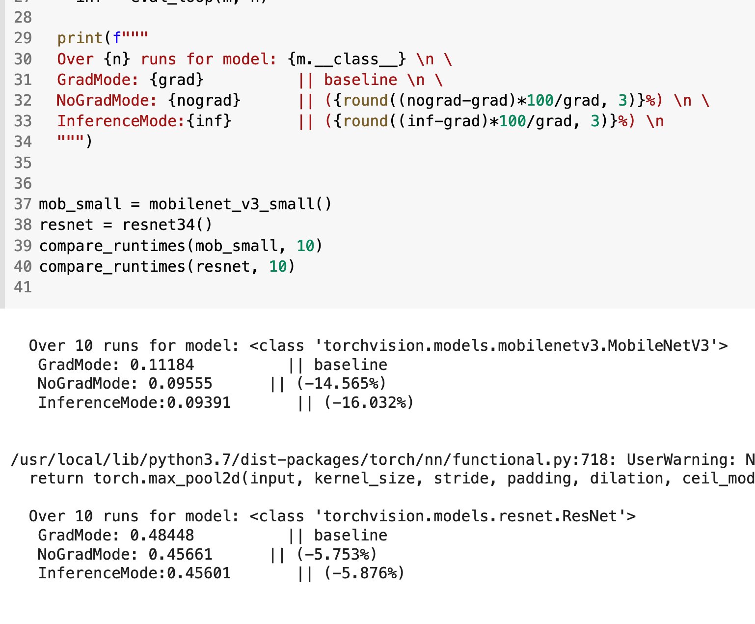
Screenshot taken from PyTorch's official tweet made on Sep 25, 2021. Link.
While NoGrad excludes operations from being tracked by Autograd, InferenceMode takes that two steps ahead, potentially speeding up your code (YMMV depending on model complexity and hardware).
nn.Linear
A module that applies an affine linear transformation to the incoming data. This transformation is represented by the formula:
where is the input, is the weight, is the bias, and is the output.
A really good example for this came up when I was trying to create a linear regression class. So, at first, I simply defined the parameters explicitly (the weight and the bias) using nn.Parameter like this:
pythonCOPIEDclass LinearRegression(nn.Module):def __init__(self):super().__init__()self.weights = nn.Parameter(torch.randn(1, dtype=torch.float),requires_grad=True)self.bias = nn.Parameter(torch.randn(1, dtype=torch.float),requires_grad=True)def forward(self, x: torch.Tensor) -> torch.Tensor:return self.weights * x + self.bias
Pretty straightforward. We explicitly create and manage weight and bias parameters. In other words, the linear transformation has been defined explicitly. I believe this is easy to understand the underlying math.
On the other hand, I could simply use nn.Linear to carry out the linear regression and leave the linear transformation and parameters' creation + management fo the nn.Module to handle on its own internally:
pythonCOPIEDclass LinearRegression(nn.Module):def __init__(self):super().__init__()self.linear_layer = nn.Linear(in_features=1,out_features=1)def forward(self, x: torch.Tensor) -> torch.Tensor:return self.linear_layer(x)
When I created a nn.Linear layer with in_features=1 and out_features=1, it's creating:
- A weight matrix of size (1, 1)
- A bias vector of size (1)
The forward pass through nn.Linear performs:
pythonCOPIEDoutput = input @ weight.t() + bias
Which, for my single-feature case, simplifies to exactly the same computation as the manual version from above:
pythonCOPIEDoutput = input * weight + bias
Which means? nn.Linear is essentially doing the same thing as the manual implementation, but in a more generalized and optimized way.
The advantage of using nn.Linear becomes more apparent when working with:
- Multiple input features
- Multiple output features
- Multiple layers
- Batch processing
In these cases, nn.Linear handles all the matrix operations and parameter management automatically, while the manual version would require significant additional code to handle these scenarios.